Guide to Extracting Data w/ APIs from the Withings Sleep Tracking Mat

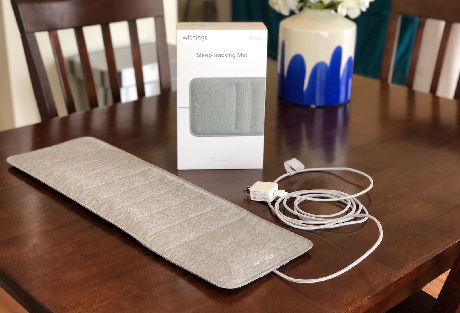
There are lots of fitness and health tracking devices that require you to strap something to your arm, finger, or head. But what if you could track your sleep without even feeling it? With the Withings Sleep Tracking Mat, a tracking mat that goes right under your mattress, you can do just that. While this notebook is meant for the tracking mat, it can be easily adapted to any other Withings product with some modifications.

If you want to know more about Withings Sleep Tracking Mat, see the README for a detailed analysis of performances, sensors, data privacy, and extraction pipelines.

TODO: fix the withings sleepmat readme url

We will be able to extract the following parameters (see the definitions at this documenation page):

Parameter Name	Sampling Frequency
Heart Rate	Every 10 minutes OR every second (when set to continuous heart rate mode)
# of REM sleep phases	Per sleep
Sleep Efficiency	Per sleep
Sleep Latency	Per sleep
Total Sleep Time	Per sleep
Total Time in bed	Per sleep
Wakeup latency	Per sleep
Waso	Per sleep
Asleepduration	Per sleep
Deep sleep duration	Per sleep
Duration to sleep	Per sleep
Duration to wakeup	Per sleep
Average heart rate	Per sleep
Max heart rate	Per sleep
Min heart rate	Per sleep
Light sleep duration	Per sleep
Night events	Per sleep
Out of bed count	Per sleep
REM sleep duration	Per sleep
Average resp rate	Per sleep
Minimal resp. rate	Per sleep
Max resp. rate	Per sleep
Sleep score	Per sleep
Total snoring time	Per sleep
Snoring episode count	Per sleep
Wakeup count	Per sleep
Wakeup duration	Per sleep

TODO: Consider adding variable names as a column to decrease confusion/searching

Note that Withings provides even more measurements than just these. You can check these out at the API reference. Since we focus on heart rate and sleep here, though, those are the main measurement types we extract.

In this guide, we sequentially cover the following five topics to extract from the Withings API: 1. Setup 2. Authentication/Authorization - This requires a couple extra steps on your part 3. Data extraction - You can get data from the API in a couple lines of code. 4. Data visualization - 4.1: We reproduce a plot for heart rate over the course of a day - 4.2: We reproduce a plot for sleep data over the course of a week 5. Data analysis - 5.1: We try to find a correlation between the length of a sleep period and the median heart rate for that sleep period. We find that the correlation is not statistically significant.

1. Setup

Relevant libraries are imported below. Just run the code to import all the libraries.

import requests
import urllib
import json
from datetime import datetime
from tqdm import tqdm

import numpy as np
import pandas as pd
import matplotlib.pyplot as plt
import seaborn as sns
from scipy.ndimage import gaussian_filter
from scipy import stats

2. Authentication/Authorization

To be able to make requests to the API, the easiest way is to use the public developer API. This section roughly follows the steps outlined here on their website.

First, follow the non-colab steps listed below:

1. Visit the developer portal and click “Open Developer Dashboard” on the top right.

2. Once logged in, click “Add an app”.

3. For now, you can just click “I don’t know” under “Services”, accept terms of use, and click “Next”.

4. Put whatever you want under “Application Name” (we used withings-test), anything under “Application Description”, and “https://wbsapi.withings.net/v2/oauth2” under Registered URLs, then click “Done”.

   • NOTE: “registered URLs” is intended to be a URL to a webserver you control and can receive requests from. However, in this notebook we are simply using it as a placeholder, as this functionality is not strictly necessary for obtaining your data.

In the end, you should see something like the below.

Now we can proceed with the rest of the notebook.

To be able to make requests to the API and extract the data we need, we need to first issue an access token. This (ephemeral) access token will serve as our key to the data. While, you don’t necessarily need to be familiar with how the issuing of the authtoken occurs, you can learn more about it by visiting the official Withings tutorial.

#@title 6. Enter your credentials below (from the application you just created)
CLIENT_ID = "d97ef704c1357d5330414a6ef6ee939062a7ef69656c51a8ab1565bc5eb4bd1e" #@param {type:"string"}
CUSTOMER_SECRET = "692001d6c0d3c915b313669fd1dbc036b9062b5c4209a25c1e5bdcf721ad7e94" #@param {type:"string"}

STATE = 'string'
ACCOUNT_URL = 'https://account.withings.com'
CALLBACK_URI = 'https://wbsapi.withings.net/v2/oauth2'


payload = {'response_type': 'code',  # imposed string by the api
    'client_id': CLIENT_ID,
    'state': STATE,
    'scope': 'user.info,user.metrics,user.activity',  # see docs (https://developer.withings.com/api-reference/#operation/oauth2-authorize) for enhanced scope
    'redirect_uri': CALLBACK_URI,  # URL of this app
    #'mode': 'demo'  # Use demo mode, DELETE THIS FOR REAL APP
}

url = f'{ACCOUNT_URL}/oauth2_user/authorize2?'

for key, value in payload.items():
    url += f'{key}={value}&'

url = url[:-1]

print(url)

https://account.withings.com/oauth2_user/authorize2?response_type=code&client_id=d97ef704c1357d5330414a6ef6ee939062a7ef69656c51a8ab1565bc5eb4bd1e&state=string&scope=user.info,user.metrics,user.activity&redirect_uri=https://wbsapi.withings.net/v2/oauth2

7. Now visit the above URL and click “Allow this app”, and copy the URL you were redirected to into the text field below. Note that if you mess up once, you have to go through the above URL again (including clicking “Allow this app”). Also, the URL is only valid for 30 seconds, so be quick!

#@title 7. Copy and paste the URL you were redirected to below
redirect_url = "https://wbsapi.withings.net/v2/oauth2?code=2669a4df72b43435ffda73401abc4d2813ae5dfa&state=string" #@param {type:"string"}

try:
    code = urllib.parse.parse_qs(urllib.parse.urlparse(redirect_url).query)['code'][0]
except Exception as e:
    print(f'Caught error:\n{e}\n')
    print("Please copy and paste the entire URL (including https)")

params = {
    'action': 'requesttoken',
    'grant_type': 'authorization_code',
    'client_id': CLIENT_ID,
    'client_secret': CUSTOMER_SECRET,
    'code': code,
    #'scope': 'user.info',
    'redirect_uri': 'https://wbsapi.withings.net/v2/oauth2'
}

out = requests.get('https://wbsapi.withings.net/v2/oauth2', data=params)

out = json.loads(out.text)

try:
    access_token = out['body']['access_token']
except KeyError as e:
    print('Took too long to paste in redirect URL. Please repeat step 7.')

Now that we have our access token, we can begin making requests to the API! This access token will last only three hours, though, so you would need to re-do step 7 if three hours pass.

3. Data extraction

Here, data extraction is pretty simple! We’ve made it possible to get all heart rate and sleep data in one function call each.

If you need to customize this part further and need to dig into the code, notice that all we need to do is make a few GET requests with the right query parameters. See the overall health data API page or the “Measure” endpoints specifically for more info.

#@title Enter start and end dates
start_date = "2020-03-28" #@param {type:"date"}
end_date = "2022-05-28" #@param {type:"date"}

num_to_description = {1: 'Weight (kg)',
                      4: 'Height (meter)',
                      5: 'Fat Free Mass (kg)',
                      6: 'Fat Ratio (%)',
                      8: 'Fat Mass Weight (kg)',
                      9: 'Diastolic Blood Pressure (mmHg)',
                      10: 'Systolic Blood Pressure (mmHg)',
                      11: 'Heart Pulse (bpm) - only for BPM and scale devices',
                      12: 'Temperature (celsius)',
                      54: 'SP02 (%)',
                      71: 'Body Temperature (celsius)',
                      73: 'Skin Temperature (celsius)',
                      76: 'Muscle Mass (kg)',
                      77: 'Hydration (kg)',
                      88: 'Bone Mass (kg)',
                      91: 'Pulse Wave Velocity (m/s)',
                      123: 'VO2 max is a numerical measurement of your body’s ability to consume oxygen (ml/min/kg).',
                      135: 'QRS interval duration based on ECG signal',
                      136: 'PR interval duration based on ECG signal',
                      137: 'QT interval duration based on ECG signal',
                      138: 'Corrected QT interval duration based on ECG signal',
                      139: 'Atrial fibrillation result from PPG'}

NUM_RETRIES = 5

def fetch_all_wrapper(endpoint_url, data, headers, arr_key, parse_data=lambda x: x):
    # wrapper around public API that retrieves arbitrarily large # of
    # records, since there is a restriction of # of records per API response
    # NOTES:
    # out['body'][arr_key] is concatenated across several requests
    # parse_data is a function that parses the returned array

    cur_offset = 0
    arr_complete = None

    while True:
        # endpoint can be flaky if the response payload is extremely large,
        # so retry at most NUM_RETRIES times
        for i in range(NUM_RETRIES):
            data_args = {
                **data,
                'offset': cur_offset
            }
            out = requests.post(endpoint_url, data=data_args, headers=headers)

            out = json.loads(out.text)

            if out['status'] == 401:
                raise Exception(f'request response is {out} for request {data_args} to endpoint {endpoint_url}, headers {headers}')

            try:
                arr = parse_data(out['body'][arr_key])
                break
            except KeyError:
                if 'body' in out.keys():
                    raise Exception(f'got key {arr_key}, expected one of {out["body"].keys()}')
                elif out['status'] == 2555:
                    # when the payload is too large, this is the status code
                    continue
                else:
                    raise Exception(f'request response is {out} for request {data_args} to endpoint {endpoint_url}, headers {headers}')

        # for example, https://developer.withings.com/api-reference/#operation/measurev2-getactivity
        # vs. https://developer.withings.com/api-reference/#operation/measure-getmeas
        if type(arr) == type({}):
            if arr_complete is None:
                arr_complete = dict()

            arr_complete.update(arr)

        elif type(arr) == type([]):
            if arr_complete is None:
                arr_complete = []

            arr_complete += arr

        # continue if there's still more to get
        if 'more' in out['body'].keys() and out['body']['more'] == 1:
            cur_offset = out['body']['offset']
        else:
            break

    # replace with concatenated version
    out['body'][arr_key] = arr_complete

    return out

def fetch_all_heart_rate(start='2020-03-10', end='2022-05-28'):
    # get all dates heart rate was collected for
    out = fetch_all_wrapper('https://wbsapi.withings.net/v2/measure', {
        'action': 'getactivity',
        'startdateymd': start,
        'enddateymd': end,
        'data_fields': 'hr_average'
    }, {'Authorization': f'Bearer {access_token}'},
        arr_key='activities')

    dates = [act['date'] for act in out['body']['activities']]

    # now for each date get the heart rate data and store as list of dicts
    dict_list = []
    for date in tqdm(dates):
        out = fetch_all_wrapper('https://wbsapi.withings.net/v2/measure', {
            'action': 'getintradayactivity',
            'startdate': int(datetime.strptime(date, '%Y-%m-%d').timestamp()),
            'enddate': int(datetime.strptime(date, '%Y-%m-%d').timestamp()) + 24 * 3600,
            'data_fields': 'heart_rate'
        }, {'Authorization': f'Bearer {access_token}'},
            arr_key='series')

        dict_list += [{'datetime': datetime.fromtimestamp(int(k)), **v} for k,v in out['body']['series'].items()]

    df = pd.DataFrame.from_dict(dict_list)

    return df


def fetch_all_sleeps(start='2020-03-10', end='2022-05-28'):
    out = fetch_all_wrapper('https://wbsapi.withings.net/v2/sleep', {
        'action': 'getsummary',
        'startdateymd': '2020-07-01',
        'enddateymd': '2022-07-01',
        'data_fields': 'nb_rem_episodes,sleep_efficiency,sleep_latency,total_sleep_time,total_timeinbed,wakeup_latency,waso,asleepduration,deepsleepduration,durationtosleep,durationtowakeup,hr_average,hr_max,hr_min,lightsleepduration,night_events,out_of_bed_count,remsleepduration,rr_average,rr_max,rr_min,sleep_score,snoring,snoringepisodecount,wakeupcount,wakeupduration'
    }, {'Authorization': f'Bearer {access_token}'}, arr_key='series')

    df = pd.DataFrame.from_dict(out['body']['series'])

    return df

hr_df = fetch_all_heart_rate(start=start_date, end=end_date)
sleeps_df = fetch_all_sleeps(start=start_date, end=end_date)

100%|██████████| 18/18 [00:13<00:00,  1.30it/s]

hr_df

	datetime	heart_rate	model	model_id	deviceid
0	2022-05-25 14:46:46	66	None	1058	None
1	2022-05-25 14:48:07	71	None	1058	None
2	2022-05-25 14:53:27	88	None	1058	None
3	2022-05-25 14:54:17	96	None	1058	None
4	2022-05-25 14:56:41	87	None	1058	None
...	...	...	...	...	...
59641	2022-03-05 23:26:56	67	None	1058	None
59642	2022-03-05 23:30:17	68	None	1058	None
59643	2022-03-05 23:36:31	85	None	1058	None
59644	2022-03-05 23:49:32	87	None	1058	None
59645	2022-03-05 23:51:39	73	None	1058	None

59646 rows × 5 columns

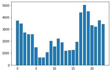
data = np.unique([(int(datetime.strftime(dt, '%H')) - 8) % 24 for dt in hr_df.datetime], return_counts=True)

plt.bar(data[0], data[1])

<BarContainer object of 24 artists>

set(hr_df.deviceid)

{None}

set(hr_df.model_id)

{1058}

set(hr_df.model)

{None}

access_token

'fafdab17e72f36fb210d40f75ab5c4995eb96a77'

!curl --header "Authorization: Bearer fafdab17e72f36fb210d40f75ab5c4995eb96a77" --data "action=getdevice" 'https://wbsapi.withings.net/v2/user   '

{"status":0,"body":{"devices":[{"type":"Sleep Monitor","battery":"high","model":"Aura Sensor V2","model_id":63,"timezone":"America\/Los_Angeles","last_session_date":1654140010,"deviceid":"4f15662709a827746ffd49b589ee37206e23e9f0","hash_deviceid":"4f15662709a827746ffd49b589ee37206e23e9f0"}]}}

json.loads('{"status":0,"body":{"devices":[{"type":"Sleep Monitor","battery":"high","model":"Aura Sensor V2","model_id":63,"timezone":"America\/Los_Angeles","last_session_date":1654140010,"deviceid":"4f15662709a827746ffd49b589ee37206e23e9f0","hash_deviceid":"4f15662709a827746ffd49b589ee37206e23e9f0"}]}}')['body']['devices']

[{'battery': 'high',
  'deviceid': '4f15662709a827746ffd49b589ee37206e23e9f0',
  'hash_deviceid': '4f15662709a827746ffd49b589ee37206e23e9f0',
  'last_session_date': 1654140010,
  'model': 'Aura Sensor V2',
  'model_id': 63,
  'timezone': 'America/Los_Angeles',
  'type': 'Sleep Monitor'}]

set(hr_df.model_id)

{1058}

set(np.array(hr_df.model))

{None}

[x for x in sleeps_df.data]

[{'deepsleepduration': 0,
  'durationtosleep': 2820,
  'durationtowakeup': 0,
  'hr_average': 61,
  'hr_max': 69,
  'hr_min': 51,
  'lightsleepduration': 3660,
  'nb_rem_episodes': 0,
  'night_events': '{"1":[0],"2":[2820],"3":[6480],"4":[6480]}',
  'out_of_bed_count': 0,
  'remsleepduration': 0,
  'rr_average': 15,
  'rr_max': 19,
  'rr_min': 12,
  'sleep_efficiency': 0.56,
  'sleep_latency': 2820,
  'sleep_score': 20,
  'snoring': 0,
  'snoringepisodecount': 0,
  'total_sleep_time': 3660,
  'total_timeinbed': 6480,
  'wakeup_latency': 0,
  'wakeupcount': 0,
  'wakeupduration': 2820,
  'waso': 0},
 {'deepsleepduration': 1620,
  'durationtosleep': 1920,
  'durationtowakeup': 0,
  'hr_average': 67,
  'hr_max': 79,
  'hr_min': 53,
  'lightsleepduration': 6300,
  'nb_rem_episodes': 2,
  'night_events': '{"1":[0,14760,1440,1980,840],"2":[1920,13800,4800],"3":[13200,2700,4920],"4":[13200,2700,600,2460,1860]}',
  'out_of_bed_count': 4,
  'remsleepduration': 3840,
  'rr_average': 15,
  'rr_max': 23,
  'rr_min': 12,
  'sleep_efficiency': 0.68,
  'sleep_latency': 1920,
  'sleep_score': 20,
  'snoring': 1140,
  'snoringepisodecount': 4,
  'total_sleep_time': 11760,
  'total_timeinbed': 17220,
  'wakeup_latency': 0,
  'wakeupcount': 2,
  'wakeupduration': 5460,
  'waso': 7140},
 {'deepsleepduration': 2940,
  'durationtosleep': 1800,
  'durationtowakeup': 1020,
  'hr_average': 66,
  'hr_max': 81,
  'hr_min': 51,
  'lightsleepduration': 12420,
  'nb_rem_episodes': 4,
  'night_events': '{"1":[0,23040],"2":[1800,21420],"3":[22620,2640],"4":[22620,3660]}',
  'out_of_bed_count': 1,
  'remsleepduration': 7500,
  'rr_average': 16,
  'rr_max': 22,
  'rr_min': 10,
  'sleep_efficiency': 0.88,
  'sleep_latency': 1800,
  'sleep_score': 62,
  'snoring': 0,
  'snoringepisodecount': 0,
  'total_sleep_time': 22860,
  'total_timeinbed': 25860,
  'wakeup_latency': 1020,
  'wakeupcount': 1,
  'wakeupduration': 3000,
  'waso': 600},
 {'deepsleepduration': 4200,
  'durationtosleep': 5220,
  'durationtowakeup': 0,
  'hr_average': 73,
  'hr_max': 88,
  'hr_min': 54,
  'lightsleepduration': 12600,
  'nb_rem_episodes': 7,
  'night_events': '{"1":[0,20400,660,360,900,1920,9240],"2":[5220,15180,1020,900,1920,9300],"3":[20220,480,1380,1740,3960,6840],"4":[20220,480,600,780,1740,9600,1200]}',
  'out_of_bed_count': 6,
  'remsleepduration': 5280,
  'rr_average': 16,
  'rr_max': 27,
  'rr_min': 10,
  'sleep_efficiency': 0.66,
  'sleep_latency': 5220,
  'sleep_score': 53,
  'snoring': 0,
  'snoringepisodecount': 0,
  'total_sleep_time': 22080,
  'total_timeinbed': 33240,
  'wakeup_latency': 0,
  'wakeupcount': 5,
  'wakeupduration': 11160,
  'waso': 7320},
 {'deepsleepduration': 0,
  'durationtosleep': 1080,
  'durationtowakeup': 0,
  'hr_average': 66,
  'hr_max': 87,
  'hr_min': 54,
  'lightsleepduration': 19560,
  'nb_rem_episodes': 6,
  'night_events': '{"1":[0,25740,780],"2":[1080,25440,1920],"3":[25380,1680,2280],"4":[25380,900,3060]}',
  'out_of_bed_count': 2,
  'remsleepduration': 6180,
  'rr_average': 15,
  'rr_max': 25,
  'rr_min': 11,
  'sleep_efficiency': 0.9,
  'sleep_latency': 1080,
  'sleep_score': 77,
  'snoring': 0,
  'snoringepisodecount': 0,
  'total_sleep_time': 25740,
  'total_timeinbed': 28740,
  'wakeup_latency': 0,
  'wakeupcount': 2,
  'wakeupduration': 3000,
  'waso': 2520},
 {'deepsleepduration': 840,
  'durationtosleep': 1200,
  'durationtowakeup': 0,
  'hr_average': 72,
  'hr_max': 79,
  'hr_min': 66,
  'lightsleepduration': 4200,
  'nb_rem_episodes': 1,
  'night_events': '{"1":[0,6960],"2":[1200,6540],"3":[5820,2820],"4":[5820,2820]}',
  'out_of_bed_count': 1,
  'remsleepduration': 480,
  'rr_average': 15,
  'rr_max': 18,
  'rr_min': 13,
  'sleep_efficiency': 0.74,
  'sleep_latency': 1200,
  'sleep_score': 20,
  'snoring': 0,
  'snoringepisodecount': 0,
  'total_sleep_time': 5520,
  'total_timeinbed': 7500,
  'wakeup_latency': 0,
  'wakeupcount': 1,
  'wakeupduration': 1980,
  'waso': 1920},
 {'deepsleepduration': 3720,
  'durationtosleep': 840,
  'durationtowakeup': 0,
  'hr_average': 69,
  'hr_max': 84,
  'hr_min': 54,
  'lightsleepduration': 6840,
  'nb_rem_episodes': 2,
  'night_events': '{"1":[0],"2":[840],"3":[15000],"4":[15000]}',
  'out_of_bed_count': 0,
  'remsleepduration': 3600,
  'rr_average': 15,
  'rr_max': 19,
  'rr_min': 12,
  'sleep_efficiency': 0.94,
  'sleep_latency': 840,
  'sleep_score': 21,
  'snoring': 0,
  'snoringepisodecount': 0,
  'total_sleep_time': 14160,
  'total_timeinbed': 15000,
  'wakeup_latency': 0,
  'wakeupcount': 0,
  'wakeupduration': 840,
  'waso': 0}]

sleeps_df

	id	timezone	model	model_id	hash_deviceid	startdate	enddate	date	data	created	modified
0	2773588367	America/Los_Angeles	32	63	4f15662709a827746ffd49b589ee37206e23e9f0	1653557580	1653564060	2022-05-26	{'wakeupduration': 2820, 'wakeupcount': 0, 'du...	1653564132	1653572591
1	2775493636	America/Los_Angeles	32	63	4f15662709a827746ffd49b589ee37206e23e9f0	1653640260	1653661080	2022-05-27	{'wakeupduration': 5460, 'wakeupcount': 2, 'du...	1653653590	1653668471
2	2777458259	America/Los_Angeles	32	63	4f15662709a827746ffd49b589ee37206e23e9f0	1653724920	1653751200	2022-05-28	{'wakeupduration': 3000, 'wakeupcount': 1, 'du...	1653747687	1653758589
3	2779030725	America/Los_Angeles	32	63	4f15662709a827746ffd49b589ee37206e23e9f0	1653806400	1653841020	2022-05-29	{'wakeupduration': 11160, 'wakeupcount': 5, 'd...	1653826737	1653848443
4	2780933603	America/Los_Angeles	32	63	4f15662709a827746ffd49b589ee37206e23e9f0	1653891420	1653920760	2022-05-30	{'wakeupduration': 3000, 'wakeupcount': 2, 'du...	1653916917	1653928152
5	2782467827	America/Los_Angeles	32	63	4f15662709a827746ffd49b589ee37206e23e9f0	1653984480	1653993120	2022-05-31	{'wakeupduration': 1980, 'wakeupcount': 1, 'du...	1653990372	1654000512
6	2784302567	America/Los_Angeles	32	63	4f15662709a827746ffd49b589ee37206e23e9f0	1654060980	1654075980	2022-06-01	{'wakeupduration': 840, 'wakeupcount': 0, 'dur...	1654076118	1654083370

Now that we’ve got dataframes with data, we can see the data they have. In particular, we have a ton of measurements from a non-ScanWatch device, so we’ll get rid of those. Note that it is theoretically possible to have another ScanWatch device (and maybe the model name will be ScanWatch2, or something different), but we were unable to test this, so if you switch between devices you might want to be careful here.

hr_df = hr_df.drop(np.where(hr_df.model != 'ScanWatch')[0])
hr_df

	datetime	heart_rate	model	model_id	deviceid
0	2022-05-17 03:37:55	84	ScanWatch	93	4518d7c4c7ba897fc5c45ed81933452a061606cd
1	2022-05-17 03:38:25	96	ScanWatch	93	4518d7c4c7ba897fc5c45ed81933452a061606cd
2	2022-05-17 03:38:57	100	ScanWatch	93	4518d7c4c7ba897fc5c45ed81933452a061606cd
3	2022-05-17 03:43:43	96	ScanWatch	93	4518d7c4c7ba897fc5c45ed81933452a061606cd
4	2022-05-17 03:53:08	103	ScanWatch	93	4518d7c4c7ba897fc5c45ed81933452a061606cd
...	...	...	...	...	...
2197	2022-05-28 22:53:38	69	ScanWatch	93	4518d7c4c7ba897fc5c45ed81933452a061606cd
2198	2022-05-28 23:03:13	71	ScanWatch	93	4518d7c4c7ba897fc5c45ed81933452a061606cd
2199	2022-05-28 23:13:11	80	ScanWatch	93	4518d7c4c7ba897fc5c45ed81933452a061606cd
2200	2022-05-28 23:43:32	94	ScanWatch	93	4518d7c4c7ba897fc5c45ed81933452a061606cd
2201	2022-05-28 23:54:01	95	ScanWatch	93	4518d7c4c7ba897fc5c45ed81933452a061606cd

2202 rows × 5 columns

And now we have just 2k rows!

4. Data Visualization

In this section, you’ll expect to see a couple plots from the Health Mate mobile app reproduced.

4.1: Heart rate single day

First, we’ll reproduce the below plot you can find in the Health Mate mobile app that displays heart rate data over the course of a single day.

Above is a plot taken from the official Withings mobile app.

#@title Enter date
date = "2022-05-20" #@param {type:"date"}
from matplotlib.ticker import FormatStrFormatter
import matplotlib.dates as dates
import matplotlib.transforms

from dateutil import tz
from scipy.interpolate import make_interp_spline
from datetime import timedelta

# measurements are taken every 10 minutes, displayed on app every 30
HEART_RATE_RECORDING_LENGTH = 30 * 60

with plt.style.context('dark_background'):
    # get the start and end times as timestamps by using the datetime library
    start_ts = datetime.strptime(date + ' 00:00:00-07:00', '%Y-%m-%d %H:%M:%S%z').timestamp()
    #end_ts = datetime.strptime(date + ' 23:59:59-07:00', '%Y-%m-%d %H:%M:%S%z').timestamp()
    end_ts = start_ts + 24 * 3600 + 30 * 60  # 00:30 the next day
    #end_ts = datetime.strptime('2022-05-25 00:30:00-07:00', '%Y-%m-%d %H:%M:%S%z').timestamp()

    # now find the indices in hr_df.timestamp that match as closely as possible
    start_idx = np.argmin(np.abs(hr_df.datetime.apply(lambda x: x.timestamp()) - start_ts))
    end_idx = np.argmin(np.abs(hr_df.datetime.apply(lambda x: x.timestamp()) - end_ts))

    x = hr_df.datetime.iloc[start_idx:end_idx]
    y = hr_df.heart_rate.iloc[start_idx:end_idx]

    # make it not as bumpy with gaussian filter. note that this does not reproduce
    # the curve exactly, as I'm not sure what smoothing algorithm they used...
    y = gaussian_filter(y, sigma=3)

    fig = plt.figure(figsize=(18,6), facecolor='black')

    x_timestamp = np.array([x_.timestamp() for x_ in x])

    # get the gaps. we include [6] as well because when you do np.diff,
    # it actually leaves out exactly one element
    differences = np.concatenate((np.diff(x_timestamp), [60 * 10]))

    # interpret a gap (i.e. when a user takes off the device for some prolonged
    # period of time) as any two measurements that are taken more than
    # 6 * 2 = 12 seconds apart, to account for minor variations around 6s
    gap_idxes = np.where(differences > HEART_RATE_RECORDING_LENGTH * 2)[0]

    # get the sleeps
    sleep_idxes = []
    for lower, upper in zip(sleeps_df.startdate, sleeps_df.enddate):
        if lower < start_ts or upper > end_ts:
            continue
        # get the location in the timestamp array that is closest to `lower`
        lower_idx = np.argmin(np.abs((x_timestamp - lower) - 0))
        # get the location in the timestamp array that is closest to `upper`
        upper_idx = np.argmin(np.abs((x_timestamp - upper) - 0))

        sleep_idxes.append((lower_idx, upper_idx))

    # first, we just plot the entire thing
    plt.plot(x, y, linewidth=3, color='#85a6f7')

    # now we overlay sleeps
    for sleep_start, sleep_end in sleep_idxes:
        plt.plot(x[sleep_start:sleep_end], y[sleep_start:sleep_end], linewidth=3, color='#3E414C')

        plt.axvline(x=x.iloc[sleep_start], linestyle='--', linewidth=1.5, color='#2F303A')

        plt.axvline(x=x.iloc[sleep_end], linestyle='--', linewidth=1.5, color='#2F303A')

    # now we overlay gaps by overlaying with white
    for gap_idx in gap_idxes:
        plt.plot(x[gap_idx:gap_idx+2], y[gap_idx:gap_idx+2], linewidth=5, color='black')

    plt.ylim(40, 180)
    plt.xlim(x.iloc[0], x.iloc[-1] - pd.Timedelta(minutes=30))

    datetimes = [
        datetime.strptime(date + ' 00:00:00-0700', '%Y-%m-%d %H:%M:%S%z'),
        datetime.strptime(date + ' 04:00:00-0700', '%Y-%m-%d %H:%M:%S%z'),
        datetime.strptime(date + ' 08:00:00-0700', '%Y-%m-%d %H:%M:%S%z'),
        datetime.strptime(date + ' 12:00:00-0700', '%Y-%m-%d %H:%M:%S%z'),
        datetime.strptime(date + ' 16:00:00-0700', '%Y-%m-%d %H:%M:%S%z'),
        datetime.strptime(date + ' 20:00:00-0700', '%Y-%m-%d %H:%M:%S%z'),
        datetime.strptime(date + ' 00:00:00-0700', '%Y-%m-%d %H:%M:%S%z') + timedelta(days=1)
    ]

    plt.xticks(ticks=datetimes, labels=['12AM', '4AM', '8AM', '12PM', '4PM', '8PM', '12AM'])

    # get the y-axis ticks to appear on the right
    plt.gca().yaxis.tick_right()

    #plt.gca().grid(axis='x', color='#2F303A')
    plt.gca().grid(axis='y', color='#2F303A', which='major')

    # hide x-axis and make the xtick labels 16 size
    plt.tick_params(
        axis='x',          # changes apply to the x-axis
        which='both',      # both major and minor ticks are affected
        bottom=False,      # ticks along the bottom edge are off
        labelsize=16,
        labelcolor='silver'
    )

    # hide y-axis and make the ytick labels 16 size
    plt.tick_params(
        axis='y',          # changes apply to the x-axis
        which='both',      # both major and minor ticks are affected
        right=False,      # ticks along the bottom edge are off
        labelsize=16,
        labelcolor='silver'
    )

    # add offset to y-axis tick labels to make them appear above gridlines
    # instead of to the side
    # https://stackoverflow.com/questions/28615887/how-to-move-a-tick-label-in-matplotlib
    dx = -50/72.; dy = 15/72.
    offset = matplotlib.transforms.ScaledTranslation(dx, dy, fig.dpi_scale_trans)
    for label in plt.gca().yaxis.get_majorticklabels():
        label.set_transform(label.get_transform() + offset)

    # turn off all borders
    plt.gca().spines['left'].set_visible(False)
    plt.gca().spines['right'].set_visible(False)
    plt.gca().spines['top'].set_visible(False)
    plt.gca().spines['bottom'].set_visible(False)

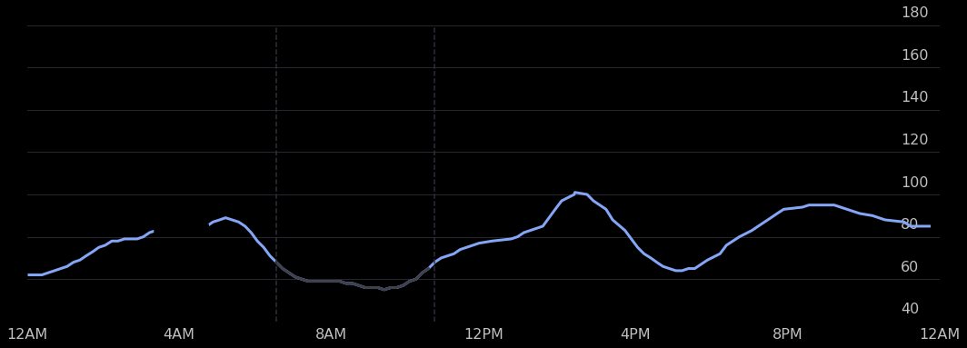
Above is a plot we created ourselves!

4.2: Sleeps over the course of a week

Now let’s try to reproduce the plot below. We can do this by taking creative advantage of matplotlib’s boxplot functionality.

The above plot is taken directly from the mobile app.

#@title Insert start of week (must be a Monday) and timezone name

week_start = "2022-05-23" #@param {type:"date"}
timezone_name = "America/Los_Angeles" #@param {type:"string"}

from matplotlib.ticker import FormatStrFormatter
import matplotlib.dates as dates
import matplotlib.transforms
import matplotlib.patches as patches
from matplotlib.ticker import (MultipleLocator, FormatStrFormatter,
                               AutoMinorLocator)

from dateutil import tz
from scipy.interpolate import make_interp_spline

from datetime import timezone
import pytz

def timestamp_to_hour_min(timestamp, tz_name='America/Los_Angeles'):
    # convert timezone to '%H:%M' in local timezone

    local_tz = pytz.timezone(tz_name)
    return datetime.fromtimestamp(int(timestamp)).replace(tzinfo=timezone.utc).astimezone(local_tz).strftime('%H:%M')

def hour_min_to_vert_pos(hour_min):
    num_mins = (int(hour_min.split(':')[0]) * 60 + int(hour_min.split(':')[1]))
    vert_dist = (16 * 60 - num_mins) / (16 * 60)

    return vert_dist

# measurements are taken every 10 minutes, displayed on app every 30
HEART_RATE_RECORDING_LENGTH = 30 * 60

NUM_DAYS = 7
RECT_WIDTH = 0.02
RECTS_START = 0.1
RECTS_END = 0.9

# add on timezone
timezone_offset = datetime.now(pytz.timezone(timezone_name)).strftime('%z')
week_start = week_start + timezone_offset
week_start_ts = datetime.strptime(week_start, '%Y-%m-%d%z').timestamp()

with plt.style.context('dark_background'):
    fig, ax = plt.subplots(figsize=(18,6), facecolor='black')

    for day_num in range(NUM_DAYS):
        rect_center_pos = RECTS_START + day_num / (NUM_DAYS-1) * (RECTS_END - RECTS_START)
        # zorder to ensure it is drawn behind rect
        plt.axvline(x=rect_center_pos, linestyle='--', linewidth=1.5, color='#2F303A', zorder=0)

        # rounded rectangles
        # https://stackoverflow.com/questions/58425392/bar-chart-with-rounded-corners-in-matplotlib

        day_ts = week_start_ts + day_num * 24 * 3600

        row = sleeps_df[np.logical_and(sleeps_df.startdate > day_ts, sleeps_df.enddate < day_ts + 24 * 3600)]

        # get the one with the longest sleep, this is how withings does it
        # source: https://support.withings.com/hc/en-us/community/posts/360026177173-Naps-don-t-count-for-sleep-tracking
        try:
            row = row.iloc[np.argmax(row.enddate - row.startdate)]
        except ValueError:
            continue

        start, end = timestamp_to_hour_min(row.startdate, tz_name=timezone_name), timestamp_to_hour_min(row.enddate, tz_name=timezone_name)

        top_pos, bottom_pos = hour_min_to_vert_pos(start), hour_min_to_vert_pos(end)

        if row.data['sleep_score'] < 50:
            color = '#ff7455'
        elif row.data['sleep_score'] < 75:
            color = '#FEDF00'
        else:
            color = '#24ffa4'

        rect = patches.FancyBboxPatch((rect_center_pos - RECT_WIDTH / 2, bottom_pos),
                                      RECT_WIDTH, top_pos - bottom_pos,
                                      boxstyle="round,pad=-0.0040,rounding_size=0.015",
                                      linewidth=3, fc=color, ec='none')

        ax.add_patch(rect)

    # get the sleeps
    sleep_idxes = []
    for lower, upper in zip(sleeps_df.startdate, sleeps_df.enddate):
        #if sleeps_df.startdate
        sleep_idxes.append((lower_idx, upper_idx))

    # now we overlay sleeps
    for sleep_start, sleep_end in sleep_idxes:
        continue

    datetimes = [
        datetime.strptime('2022-05-24 00:00:00-0700', '%Y-%m-%d %H:%M:%S%z'),
        datetime.strptime('2022-05-24 04:00:00-0700', '%Y-%m-%d %H:%M:%S%z'),
        datetime.strptime('2022-05-24 08:00:00-0700', '%Y-%m-%d %H:%M:%S%z'),
        datetime.strptime('2022-05-24 12:00:00-0700', '%Y-%m-%d %H:%M:%S%z'),
        datetime.strptime('2022-05-24 16:00:00-0700', '%Y-%m-%d %H:%M:%S%z'),
        datetime.strptime('2022-05-24 20:00:00-0700', '%Y-%m-%d %H:%M:%S%z'),
        datetime.strptime('2022-05-25 00:00:00-0700', '%Y-%m-%d %H:%M:%S%z')
    ]

    #plt.xticks(ticks=datetimes, labels=['12AM', '4AM', '8AM', '12PM', '4PM', '8PM', '12AM'])
    plt.xticks(ticks=np.linspace(0.1,0.9,NUM_DAYS), labels=['Mon', 'Tue', 'Wed', 'Thu', 'Fri', 'Sat', 'Sun'])
    plt.yticks(ticks=np.linspace(0, 1, 5), labels=['4PM', '12PM', '8AM', '4AM', '12AM'])

    # get the y-axis ticks to appear on the right
    plt.gca().yaxis.tick_right()

    #plt.gca().grid(axis='x', color='#2F303A')
    #plt.gca().yaxis.set_minor_locator(MultipleLocator(5*4))
    #plt.gca().yaxis.set_minor_locator(MultipleLocator(5 * 8))
    plt.gca().yaxis.set_minor_locator(AutoMinorLocator(n=2))
    plt.gca().grid(axis='y', color='#2F303A', which='both')

    # hide x-axis and make the xtick labels 16 size
    plt.tick_params(
        axis='x',          # changes apply to the x-axis
        which='both',      # both major and minor ticks are affected
        bottom=False,      # ticks along the bottom edge are off
        labelsize=16,
        labelcolor='silver'
    )

    # hide y-axis and make the ytick labels 16 size
    plt.tick_params(
        axis='y',          # changes apply to the x-axis
        which='both',      # both major and minor ticks are affected
        right=False,      # ticks along the bottom edge are off
        labelsize=16,
        labelcolor='silver'
    )

    # add offset to y-axis tick labels to make them appear above gridlines
    # instead of to the side
    # https://stackoverflow.com/questions/28615887/how-to-move-a-tick-label-in-matplotlib
    dx = -50/72.; dy = 15/72.
    offset = matplotlib.transforms.ScaledTranslation(dx, dy, fig.dpi_scale_trans)
    for label in plt.gca().yaxis.get_majorticklabels():
        label.set_transform(label.get_transform() + offset)

    start_day_fmted = datetime.strftime(datetime.strptime(week_start, '%Y-%m-%d%z'), '%b %d')
    end_day_fmted = datetime.strftime(datetime.strptime(week_start, '%Y-%m-%d%z') + timedelta(days=7), '%b %d')
    plt.title(f'{start_day_fmted} - {end_day_fmted}', size=20, pad=40)

    plt.gca().set_axisbelow(True)
    # turn off all borders
    plt.gca().spines['left'].set_visible(False)
    plt.gca().spines['right'].set_visible(False)
    plt.gca().spines['top'].set_visible(False)
    plt.gca().spines['bottom'].set_visible(False)

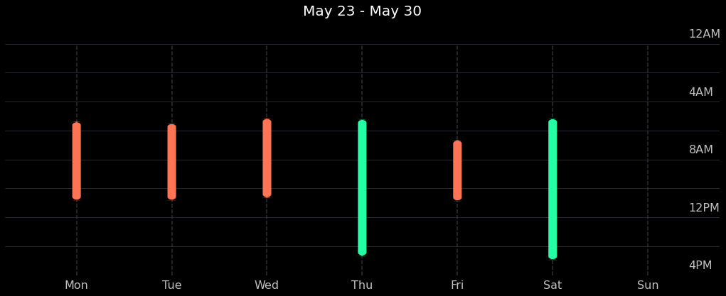
Looks like we were able to pretty accurately reproduce the same things you can see in the mobile app by querying the public API!

5. Data Analysis

Data isn’t much without some analysis, so we’re going to do some in this section.

DISCLAIMER: the analyses below may not be 100% biologically or scientifically grounded; the code is here to assist in your process, if you are interested in asking these kinds of questions.

5.1: Heart rate vs. sleep period length

Maybe the heart rate is correlated with how long a particular sleep period was. Let’s see if this hypothesis is true.

#@title Set date range and timezone
start = "2020-01-01" #@param {type:"date"}
end = "2022-05-22" #@param {type:"date"}
timezone = "US/Pacific" #@param {type:"string"}
params_all = {
    'start': f'{start}T00:00:00.000Z',
    'end': f'{end}T00:00:00.000Z'
}

First we get the length of each sleep in hours.

sleeps_df['Length (hours)'] = (sleeps_df.enddate - sleeps_df.startdate) / 3600

Next we get the median heart rate for each sleep.

measurement_timestamps = hr_df.datetime.apply(lambda x: x.timestamp())

all_heart_rates = []
median_heart_rates = []

for sleep_start, sleep_end in zip(sleeps_df.startdate, sleeps_df.enddate):
    idxes = np.where(np.logical_and(measurement_timestamps > sleep_start, measurement_timestamps < sleep_end))[0]

    heart_rates = np.array(hr_df.iloc[idxes].heart_rate)

    all_heart_rates.append(heart_rates)
    median_heart_rates.append(np.median(heart_rates))

sleeps_df['Median heart rate'] = median_heart_rates

Let’s make a quick plot to get some intuition. Here we just use seaborn, as it’s very quick to get beautiful plots out with minimal effort.

p = sns.jointplot(x='Length (hours)', y='Median heart rate', data=sleeps_df, kind='reg')

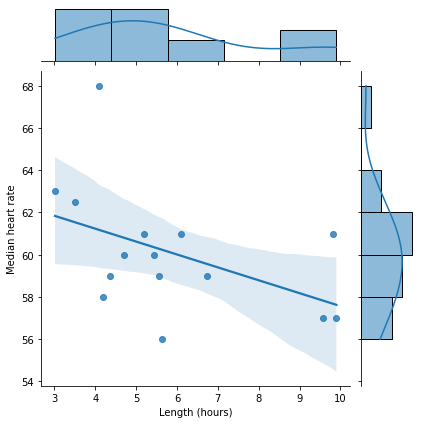
As we can see from the scatterplot above, it looks like there might be a correlation there. Let’s compute \(R^2\) just to see exactly how correlated.

We’ll follow this documentation and perform a linear regression to obtain the coefficient of determination.

from scipy import stats
slope, intercept, r_value, p_value, std_err = stats.linregress(sleeps_df['Length (hours)'], sleeps_df['Median heart rate'])

print(f'Slope: {slope:.3g}')
print(f'Coefficient of determination: {r_value**2:.3g}')
print(f'p-value: {p_value:.3g}')

Slope: -0.611
Coefficient of determination: 0.214
p-value: 0.0825

We also see that the p-value, which is determined by scipy to be the two-sided p-value for a hypothesis test whose null hypothesis is that the slope is zero, is not significant (>0.05).